
PCA, visualized for human beings
Principal Component Analysis (PCA) is often described by intro machine learning courses as follows:
- Dimensionality reduction.
- Decorrelation of features.
- Singular Value Decomposition / matrix factorization:
- Projecting the data onto a subspace spanned by the top N eigenvectors of the feature covariance matrix.
That’s alot of unhelpful words for someone who is new to the topic. I think we can build a better intuition for these ideas, with a few animations to help. PCA can be used for many types of data, but we’ll focus on images here.
I’ll assume a high-school understanding of statistics and linear algebra - nothing more.
| These animations were created using a fork of manim - a super-cool Python library by the guy at 3blue1brown. Here's a fun Twitter shoutout about it! |
- The covariance matrix of an image
- What if we had more ’s?’
- Calculating
- Calculating
- A thought experiment: filling in a canvas
- If we think of the covariance matrix as a transformation, what does it do?
- So what are the eigenvectors of the covariance matrix?
- So that’s why we use eigenvectors as a new basis…
- Decorrelation and dimensionality reduction
- How to find these eigenvectors, and how much of each eigenvector do we use?
The covariance matrix of an image
What is the covariance matrix of an image? Let’s start with its definition.
Say we have , a single image, flattened from a square . As an example, if we started with a square image, we would flatten to a single row of pixels.

To keep things simple, assume we have no color channels (like RGB). This is a grayscale image, with a single value from 0 to 255 for each pixel. We can then normalize this scale to fall between 0 and 1.1
An image X could then be represented with something like this: a dimensional vector.
Ok, cool. So what’s the covariance matrix?
Let’s ask Wikipedia. For a single pair of pixels and , it is:
In general we can write this as a dot product:
Wait a second…expectation? ?
Aren’t we just talking about a single image right now?
Indeed, if we only had a single image, would be exactly equal to . And would be exactly equal to . It wouldn’t be meaningful to calculate covariance for a single image, just like it wouldn’t be meaningful to compute an average when you only have one sample. So let’s keep going.
What if we had more ’s?’
Let’s say we had many different observations of ’s. For example, a bunch of handwritten 2’s. observations, to be precise. A single observation of is , but let’s drop the 1 to keep things clean.
So now we have a collection of ’s which is . We’ll call this collection boldface . It looks like this:
is getting complex, so let’s agree on some notation. can be described by:
- An index which runs from 1 to , describing each of the pixels.
- Continuing with our example above, .
- We usually put as a subscript: .
- An index running from 1 to , describing each “observation”, or different image.
- We usually put as a bracketed superscript:
So, means “the value of the 3rd pixel in the 5th image”.2
Calculating
Now we can meaningfully calculate , the expected value for pixel i:
Leave it to mathematicians to come up with fancy-looking notation for a simple idea! All we are saying here is: if we take the th pixel from all N images, add up their values, and divide by N, we get the average value for pixel i. Easy.
If we do this for every pixel, we get 64 different averages. We can then pack all of these into a single vector, :
Calculating
We are trying to understand .
To start, let’s take a look at the meaning of : the covariance between a specific pixel i and specific pixel j.
For every single picture, we calculate how much its pixel i differs from the average pixel i. We also calculate how much its pixel j differs from the average pixel j.
Then we multiply these two values together, for every possible pairing of i and j! How many do we have? Why, , of course.
Our possible pairs can be neatly arranged into a square matrix like so:
How many such square matrices can we make? of them - one for each image.
Then we take the expectation, or mean value, of all N of these square matrices. That expression is equivalent to .
Note the following is true for any specific value, , from this mean matrix:
- It is large and positive if whenever pixel i is higher than average, pixel j tends to be higher than average (or vice versa).
- It is large and negative if whenever pixel i is higher than average, pixel j tends to be lower than average (or vice versa).
- It is close to zero when there’s a pretty even split between these situations. In other words, seeing a high value for pixel i doesn’t give you much useful information about pixel j - it’s higher as often as it is lower.
A thought experiment: filling in a canvas
We established above that a given gives us a measure of how “related” two pixels tend to be. If pixel i is dark, does pixel j tend to be dark as well? Or does it tend to be light? Or does it give us no information at all?
The first row of the covariance matrix, then, is all of the ’s for pixel :
So do a thought experiment with me. Let’s say I give you a blank pixel canvas, and a covariance matrix, calculated on many samples of a digit that is unknown to you. I have a hidden image of this digit, and I will reveal it to you pixel by pixel. You have to try to fill in your canvas by guessing what the image looks like.
I tell you that, for example, the 50th pixel is pure black, so you fill in pixel 50 as pure black. But can you make any guesses about the rest of the image?
Well…yes! The 50th row of the covariance matrix tells you how the rest of the pixels in the image should be related to pixel 50. If is a very negative value, this tells you that pixel 64 (in the bottom-right corner) should actually be very white. If is a very positive value, that tells you that pixel 19 should be pretty dark.
In fact, you should be able to look at every pixel in the image and fill in a “guess” for the value, based on the dark pixel #50 that you now know about.
I could continue this entire exercise by telling you about pixel 51 as well. And 52. And 53. In fact, you could go through all 64 pixels and do this for each pixel, adjusting your guesses each time. And so on until you’ve covered the whole image.
So what will you end up with? Well, let’s say the hidden image I had was a 2, and our covariance matrix was calculated using many examples of 2’s. Chances are you’ll also end up with something that looks like a 2 - because every time I gave you a pixel, you went through and filled in / erased other pixels based on the relationships that we usually tend to see in images of 2s.
Now what if the hidden image had been something very different from a 2 - say, just a black line across the top of the image? Normally we’d never expect such a black line to appear in images of 2s, so its covariance with the pixels that normally do appear in 2’s should be around zero, give or take some noise. There is no obvious relationship. If we repeat the exercise above, the output probably wouldn’t look much like a 2 - we’d likely just get some random noise by chance.
If we think of the covariance matrix as a transformation, what does it do?
Thinking back to the thought experiment above, we can observe the following. Remember that our covariance matrix was calculated using a bunch of different images of 2’s.
- Applying that covariance matrix to an image of a 2 will tend to reinforce the pixel relationships that are commonly associated with 2’s.
- Applying that covariance matrix to an image that doens’t look much like a 2 will just tend to result in noise.
Thus we can think of this covariance matrix almost like a naive child that has only ever learned to draw 2’s. If we give it something that seems consistent with a 2 - say, the top curve or that bottom straight line - it will “fill in” the rest of the image based on the pixel relationships that tend to appear in 2’s. If we give it something inconsistent with a 2, it will probably just add some meaningless noise. And if we pass in a complete 2, it will probably just make the whole thing darker.
So what are the eigenvectors of the covariance matrix?
Here’s some basic intuition about eigenvectors that we need:
- A matrix is a transformation.
- An eigenvector for the matrix is able to pass through that matrix transformation without changing direction - only magnitude.
- The corresponding eigenvalue is that change in magnitude.
(If you don’t have this intuition, stop right now and go watch this amazing video by 3blue1brown.)
So go back to the covariance matrix we found in the previous step. What are its eigenvectors?
They are images that are able to pass through the matrix without changing direction - only magnitude.
“…what do you mean by change direction?”
To be fair, the human brain is bad at visualizing things in more than 3 dimensions. So let’s think about images with only 3 pixels.
- Imagine the values [0, 0.2, 0.1], [0, 0.4, 0.2], and [0, 1.0, 0.5]. These vectors all “point” in the same direction. They only differ in magnitude:
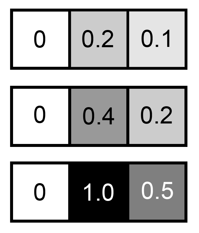
- Now imagine the values [0, 1, 1], [1, 1, 0], or [1, 0, 1]. These vectors do not point in the same direction, even though they have the same magnitude.
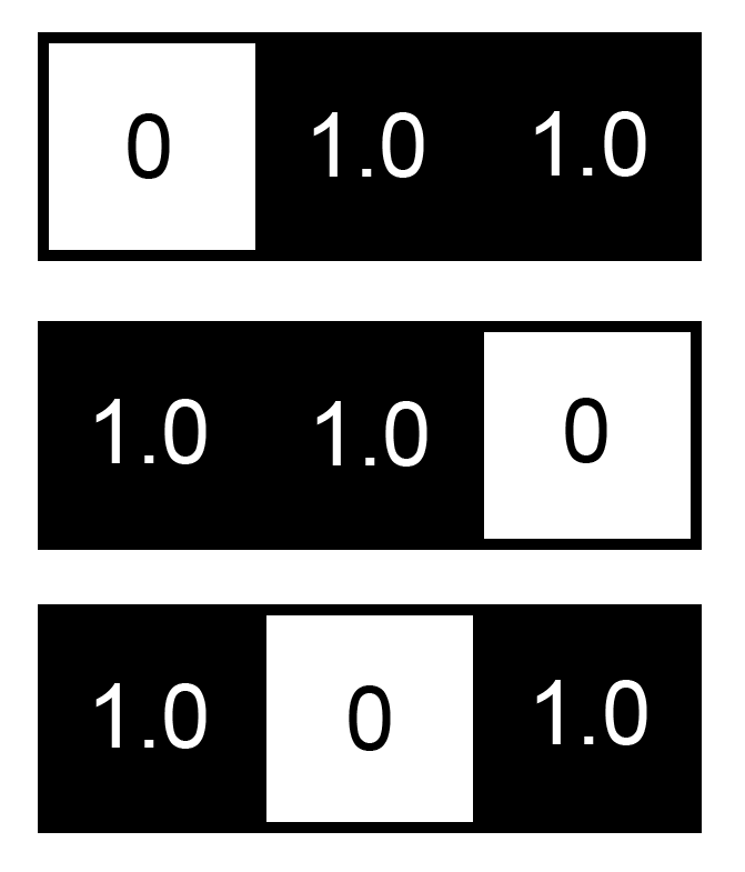
So in the context of a picture, “not changing direction” means the same pixels stay on. They may get lighter or darker, but they maintain their proportions to each other.
So that’s why we use eigenvectors as a new basis…
Now it should be a little more clear: the eigenvectors of the covariance matrix are images which are able to pass through that matrix and only get lighter or darker - but the pixel relationships do not change.
Specifically, an eigenvector with a large and positive eigenvalue will get longer - or in the context of an image, its pixels become more intense after passing through the covariance matrix.
We can imagine that if we’ve calculated our covariance matrix on a specific set of images - i.e. only a certain digit - the eigenvectors will necessarily encode structures that are very typical of that digit (at least, within your dataset).
In fact, we should be able to add a bunch of these eigenvectors up, in certain quantities, and get something that looks very much like our original image!
What are those quantities? That leads me to…
Decorrelation and dimensionality reduction
The covariance matrix was created by matrix-multiplying two identical things by each other, so it is real and symmetric (meaning, the first row is equal to the first column, second row to the second column, etc.):
Eigenvectors of real symmetric matrices are orthogonal to each other. Again, it’s hard to imagine a 90 degree angle in a space with more than 3 dimensions, but all it means is that there is no redundant information in the eigenvectors.
If we’re trying to construct our image by adding up a bunch of eigenvectors, each additional one that we throw in adds information that was not present in the others.
(If this doesn’t make sense intuitively, think of it this way: if you are at Point A and Point B is north-west of you, there is no way you can get to point B by only taking steps towards the north. You must also take some steps towards the west. We say north and west are orthogonal to each other.)
This is what it means for PCA to decorrelate features: by using eigenvectors as our new basis for representing the image, we automatically ensure that our basis is made of orthogonal vectors.
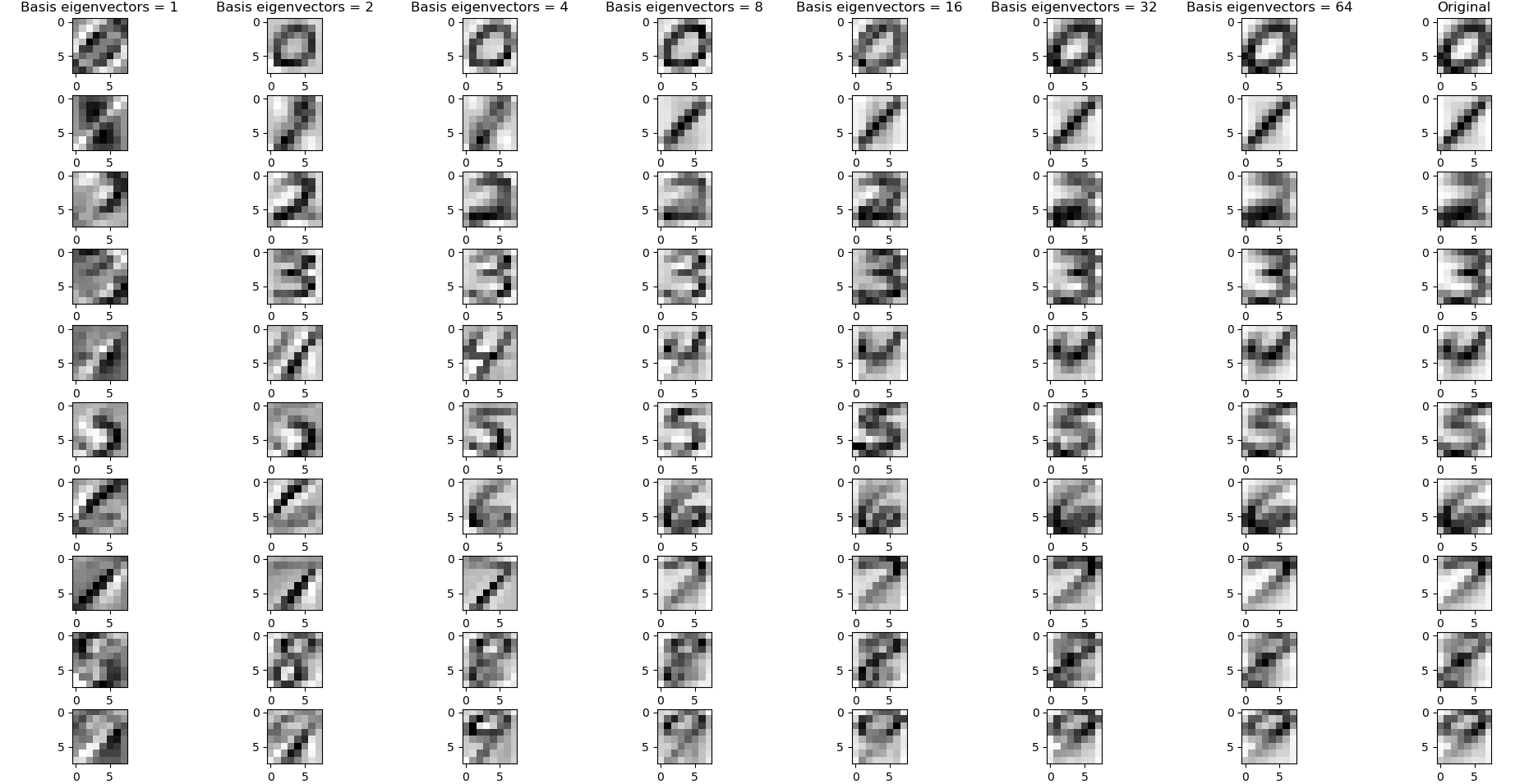
And what about dimensionality reduction? A covariance matrix will have K eigenvectors, but you certainly don’t need to use them all to get a decent reconstruction. You can obtain decent reconstructions of MNIST digits with as few as 4 eigenvectors in your basis, when the eigenvectors are calculated from class-specific data:
How to find these eigenvectors, and how much of each eigenvector do we use?
Singular Value Decomposition (SVD) refers to the operation in linear algebra that takes a matrix and factors it into the following components:
- is our original matrix that we are trying to find eigenvalues for. In this case it is the covariance matrix that we calculated from all of our images.
- U’s columns are the left singular vectors, and V’s columns are the right singular vectors. In the case of the covariance matrix which is positive semidefinite, , and its columns are the eigenvectors we wish to find.
- The values of the diagonals on are the amount by which each of these eigenvectors get transformed when they go through the transformation defined by .
Once we have , we simply take the number of eigenvectors from it that we want. (We usually take the top eigenvectors by eigenvalue.) We then “apply” (dot product) it with in order to obtain the projection of onto the new subspace spanned by our reduced (which we will call W in the code below).
Implementing this in Python is actually quite simple - here’s an example of how you might do it. The following assumes that your data has been pre-processed to be zero-centered. For an excellent explanation, check out http://cs231n.github.io/neural-networks-2/#datapre.
class Pca:
    '''
    A simple class to run PCA and store the truncated U matrix for use on the test set.
    '''

    def __init__(self):
        self.W = None

    def pca_train(self, X, n=5):
        '''
        Helper function to perform PCA on X and store the chosen eigenvectors from U.

        If input X is T x d,

        transformed X' is T x d'

        Also saves the chosen columns of U to self.W.

        Based heavily on http://cs231n.github.io/neural-networks-2/.
        '''

        # PCA down to top n eigenvectors
        # Assume input data matrix X of size [T x d]
        cov = np.dot(X.T, X) / X.shape[0] # get the data covariance matrix
        U,S,V = np.linalg.svd(cov)

        # eigenvectors are returned sorted by eigenvalue; get top n
        X_prime = np.dot(X, U[:,:n])

        # save W = U[:,:n] for use again in testing; we only train
        # PCA on the TRAIN SET to prevent data leakage!
        self.W = U[:,:n]

        return X_prime

    def pca_transform(self, X):
        '''
        Use the previously trained U to transform an input X (i.e. test data)
        '''
        assert self.W is not None, "pca_test() called when self.W is None. Did you call pca_train() first?"
        return np.dot(X, self.W)
-
Usually, represents black while represents white. For simplicity we flip this convention in the post to keep things simple: is a completely black pixel. ⤴
-
Note - this boldface notation to represent a batch of datapoints is common but certainly not standard. ML literature notation tends to be all over the place. Always read carefully. ⤴