Gaussian Discriminant Analysis, explained for human beings

This post is an extension of an answer that I wrote for a CrossValidated StackExchange question which asked someone to explain Gaussian Discriminant Analysis at a high-school level.

I really like the ELI5-type framing for questions in general, as I find that machine learning textbooks tend to trade off understandability for the layman in favour of precision. While the following may never pass muster in a proof, it was how I personally wrapped my head around the idea of GDA.

I’m going to elaborate on my answer here.

---

Andrew Ng’s notes on GDA and generative learning algorithms are the best formal explanation that I have seen of the concept, but I want to “try to explain this for someone at a high-school level” as requested (and relate it back to Andrew’s notes for those of you who care for the math).

Some fruity setup

Imagine that you have two classes of things. A class is just a category. Describe one class as $y=0$ and one class as $y=1$. I.e. if we are talking about classes of fruit, then $y=0$ could be $apples$, and $y=1$ could be $oranges$.

You have a datapoint $x$ that describes an observation of one of these things out in the wild. Say you go to the supermarket and see an apple, and you record some data about it. What might you record? Perhaps:

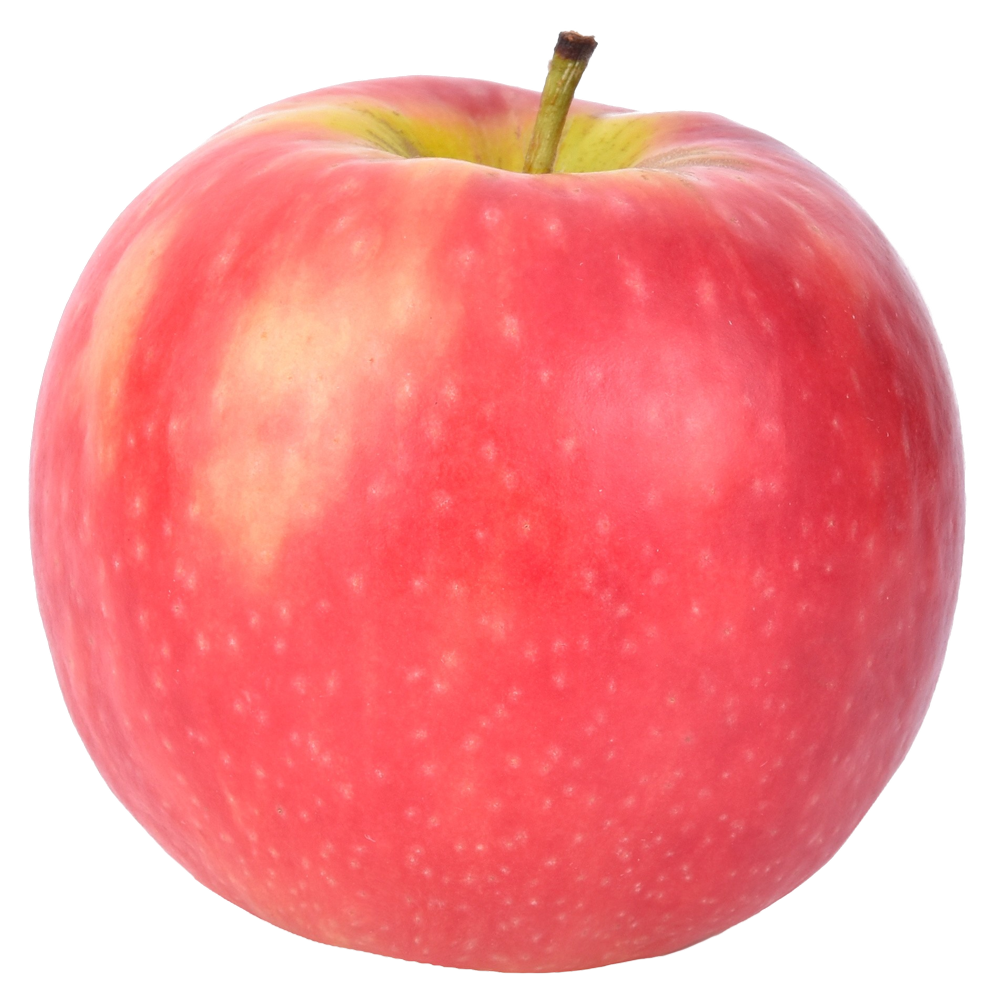
• Price, in dollars
• Diameters, in cm
• Weight, in grams
• Color - How red it is, on a scale of say, 0 to 1, where 0 is not red at all and 1 is the reddest apple possible

It can be a collection of any attributes that can be measured, in whatever units you like, and you can measure as many things to describe an $x$ as you like. You could also measure the grams of sugar in the apple, the number of bruises on it…whatever your imagination might come up with.

However, if we’re using GDA, the thing that you’re measuring should be normally distributed. Why? We’ll come back to that.

(But this means you shouldn’t define color in a way such as $red=0$, $green=1$, $yellow=2$, $blue=3$. There is no reason why color values, defined in such a way, should be normally distributed among all apples.)

Say we stick with the example above and measure these 4 different things to describe an $x$. Then we say that our $x$ is 4-dimensional. In general we say that $x$ is $d$-dimensional.

An observation could be, then:

$$[price=5,diameter=10,weight=98,color=0.5]$$

In shorthand we describe this specific apple observation as:

$$x = [5, 10, 98, 0.5]$$

Every time we see an apple, we can record it by writing down such an $x$. We’ll observe $x_1$, $x_2$, $x_3$…etc etc.

We can also average over all our observations of x to come up with a $\mu_x$. This describes the average apple on all these dimensions, within the context of the apples that we have seen.

$$\mu_x = [price_\textrm{mean}, diameter_\textrm{mean}, weight_\textrm{mean}, color_\textrm{mean}]$$

And we can do this same exercise for oranges. Bear all this in mind for the next part…

Introducing GDA

Here’s the model of GDA from Andrew’s notes:

Credit: Andrew Ng

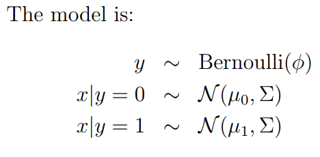
Let’s translate these lines into plain English:

Line 1: $y \sim Bernoulli(\phi)$

$p(y)$ is the chance that a fruit is either an apple $(y=0)$ or orange $(y=1)$.

This chance can be described as an unfair coin-flip, and $\phi$ is the chance of us getting heads. We’ll say for the sake of argument that heads represents apples; then $\phi = 0.4$.

(You could just as easily have heads represent oranges, but then $\phi = 0.6$).

Why an unfair coin flip? Well, it should represent something about the nature of the underlying process that generates fruit in our world. Perhaps we live in a world where we only grow apples and oranges, and orange farms are a little bit more popular than apple farms. In fact, there is a 40% chance that any given fruit is an apple, and therefore a 60% chance that any given fruit is an orange. We write this as:

$$p(y=0)=0.4$$

and

$$p(y=1)=0.6$$

Line 2: $x|y = 0 \sim \mathcal{N}(\mu_0, \Sigma)$

This reads, “given y is 0, x would then be distributed Normally with mean = $\mu_0$ and a covariance matrix of $\Sigma$.

Let’s break that down.

Given y=0 (we know the thing is an apple), its typical measurements (the stuff we agreed to measure in $x$) are normally distributed according to $\mu_0$ and $\Sigma$.

Let’s start with $\mu_0$

We all have a pretty good intuition of the bell curve from high school stats, but here’s the little mental hump that you have to get over: normal distributions can exist in more than 1 dimension!

This is precisely what $/mu_0$ is describing. Recall from above that it contains 4 numbers, describing average price, diameter, weight and colour.

This is a 4-dimensional normal distribution that describes the average apple.

Likewise, $/mu_1$ is a 4-dimensional normal distribution that describes the average orange.

What about $\Sigma$?

I will assume here that you have some intuition of what a covariance matrix is.

If not, here’s a very fuzzy explanation. Think of it as a $d$x$d$ grid, where the 4 dimensions are written out across the rows and columns. Where $weight$ and $diameter$ intersect, there will be a number describing how these two things are related:

• It is positive if higher weight tends to be seen alongside higher diameter;
• It is close to 0 if the two don’t seem to be very related;
• it is negative if higher weight tends to be seen alongside lower diameter.

In the case of apples, we probably expect the covariance between weight and diameter to be positive. Large apples generally weigh more.

Aside: astute readers may observe that there are actually two places where weight and diameter intersect in this table, and they will have the same value. This is consistent with the fact that a covariance matrix is always symmetric across its main diagonal.

Can we use the same $\Sigma$ for apples and oranges?

Credit: Andrew Ng

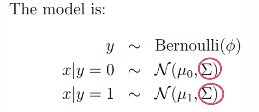
Note that in Andrew’s model, he had separate $\mu_0$ for apples and $\mu_1$ for oranges, but he uses the same $\Sigma$ for both fruit. (Well, Andrew doesn’t refer to any fruit, but we’re using them as a convenient mental device.)

This means that in our model, we have the flexibility to allow for the possibility that apples and oranges have different mean prices, weights, diameters, and colours. This makes sense intuitively: oranges are usually a little bigger, apples tend to be redder, etc.

But by using the same $\Sigma$, we assume that the way those dimensions relate to each other is the same regardless of fruit. I.e. if heavier apples tend to be bigger apples, then heavier oranges also tend to be bigger oranges.

Furthermore, we assume this is true to the same proportion for both fruits - i.e. if an apple that weighs 2x the average apple more tends to have 1.5x diameter, then an orange that weights 2x the average orange tends to have 1.5x diameter as well.

Again, for apples and oranges, this seems pretty reasonable. But this is not an inherent property of GDA. You can absolutely set up a model with separate $\Sigma_0$ and $\Sigma_1$.

(More on this in the footnote.)

Ok…after all that setup, do a thought experiment:

Flip a unfair coin that determines if something is apple or orange, to represent the underlying commoness of apples and oranges in the world.

Then, based on the fruit that we got, go to d-dimensional Normal Distribution 0 characterized by $\mathcal{N}(\mu_0, \Sigma)$, or Normal Distribution 1 characterized by $\mathcal{N}(\mu_1, \Sigma)$.

Sample a datapoint from that distribution. This is akin to actually observing an apple or orange out in the real world.

If you repeat this many times you’ll get a ton of datapoints in 𝑑-dimensional space. You’ll have seen a bunch of apples and a bunch of oranges, and you can plot their prices/weights/diameters/colours on a d-dimensional graph.

The distribution of this data, provided we have enough of it, will be “typical” of the underlying process that generates apples and oranges in our world.

(Hence why his note is called “Generative Learning algorithms”!)

But what if we do this backwards?

I give you a bunch of data instead, and I tell you that it was generated in such a fashion, but you can’t be sure which are oranges and which are apples.

You could then play around with different combinations of values in $\mu_0$, $\mu_1$, and $\Sigma$ until you get a model that “fits” the data you’ve observed.

This backwards exercise is Gaussian Discriminant Analysis!

…ok, but why is this useful?

If our model assumptions are reflective of reality, and our model fits the data well, we assume that this model is pretty reflective of the real underlying forces that determine how apples and oranges show up in our world. In machine learning parlance, we are trying to model the data generating process.

If we have the $x$ (price, diameter, weight, colour) of an unknown fruit, and are asked to guess whether it is apple or orange, we can run this exercise:

• Calculate the probability that, given the data $x$ we observed, it came from the apple distribution.
• Calculate the probability that, given the data $x$ we observed, it came from the orange distribution.

The one with the higher probability will be our guess for the mystery fruit’s identity. In machine learning jargon we call this a prediction!

(The specifics of how to do this are in Andrew’s notes, if you are curious).

---

Footnote: When we assume that $\Sigma$ is the same between classes, we have a special case of GDA called Linear Discriminant Analysis, because it results in a linear decision boundary (see pic below from Andrew’s notes):

Credit: Andrew Ng

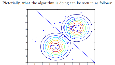
This assumption does not have to hold. GDA describes this exercise in the most general case, when $\Sigma$ can be different between classes.